Introduction
A new coronavirus called SARS-CoV-2, which causes Covid-19, surfaced a few months ago in China. The new virus affects a patient’s lungs, causing severe pneumonia, thereby increasing the risk of death, especially among the elderly or those suffering from other diseases. A major problem is that this infectious disease rapidly spreads in the population, and the high rates of infection lead to a large number of intensive care admissions. As a result, death rates are particularly high, causing a lot of fear and distress in the population, and this is even more so because presently there are no drugs or vaccine to treat this disease. At the same time, health systems in affected countries face many difficulties in tackling the high number of cases as well as in dealing with patients who need intensive care. In this scenario, in this work, we focus on forecasting death rates of patients with covid-19. The distribution of the time periods between deaths (repose periods) provides useful information about the probability that the next death will occur within some specific time interval, and thus it is very important for forecasting purposes. In general, Exponential, Binomial, and Weibull distributions are widely used in survival analyses for modeling occurrence rates. However, in a somewhat different context concerning volcanic hazard data, mixtures of exponentials 1 have been proposed in earlier literature as an alternative to the aforementioned methods; note that Exponential and Binomial distributions are not generally adequate because of the nonstationary nature of the time series involved. On the other hand, the authors have underlined the advantages of using mixtures of exponentials in comparison to a Weibull distribution. In the present study, we are also faced with nonstationary time series, as there are different regimes suggested by the data as will be shown in the sequel. In view of this, we also propose to use a mixture of exponential distributions for modeling death hazards over time due to covid-19. Results of this research could then be used for better organizing the health system (for instance, forecasting needs of hospitals with respect to numbers of ventilators, increasing intensive care units, etc.). We applied this model in the case of Italy, which is amongst the European countries most affected by the disease, with thousands of fatalities; however, the model can also be used in any heavily affected country. It is remarkable that there is a flourishing international literature on covid-19, and the case of Italy has been particularly investigated 2, 3 (e.g., reference 2 describes how the Italian government takes measures in order to contain the health risk, whereas in reference 3, a model is proposed for predicting the course of the epidemic).
Methods
The theoretical approach
Finite mixtures have been well documented in the existing literature. More specifically, a finite mixture of unknown exponential distributions with two components has a probability density function of the form 4
f(t;Λ) = pf1 (t;λ1) + (1 – p)f2 (t;λ2)
with f1(t;λ1) = λ1e(–λ1t) and f2(t;λ2) = λ2e–λ2t; Λ is the vector parameter (p,λ1,λ2); the symbol t( ≥ 0) stands for time; p is the weight of the first component and 1 – p the weight of the second component, with p > 0; f1 and f2 are the component densities, which are both exponentials with corresponding parameters λ1 > 0 and λ2 > 0, also called rate parameters or hazard rates (for our case, these will be the rate of mortality per minute). Remark that this model can also be easily generalized to include more than two components. The cumulative distribution function of a two-component mixture of exponentials takes the form F(t;Λ) = p(1 – e–λ1t) + (1 – p)(1 – e–λ2t). Then, the probability that at least a new death will occur in the next t min supposing that the last death has just occurred is a special case of equation (5) of Mendoza-Rosas and De la Cruz-Reyna 1, obtained for s = 0, and it is equal to F(t;Λ). In order to compute this probability, we need to estimate the parameters λ1 and λ2, and the weights p (and 1 – p) using the data in hand. In order to proceed, we use the idea of Mendoza-Rosas and De la Cruz-Reyna 1 for fitting a mixture model; that is, we consider the number of regimes to be the number of components of the model. Regimes can be represented graphically using the change of slope in the cumulative plot of the number of deaths.
Data collection design
Data concerning fatal cases were collected for the time period between 21 February 2020 (date of the first fatal case in Italy) and 30 April 2020, and between the 21 February 2020 and 8 May 2020 for comparison reasons using the World Health Organization database (https://bing.com/covid/local/italy).
Data classification
In the case of Italy, it appears from Figures 1 and 2, replicated from https://bing.com/covid/local/italy (see arrow for cumulative distribution function of deaths), that there are two regimes – representing the components of the mixture – which concern time periods from 21 February 2020 to 5 April 2020 (first category), corresponding to 45 days, and from 6 April 2020 onward (second category). The first category refers to increasing number of deaths on a daily basis, whereas the second one refers to number of deaths becoming stable on a daily basis and then slowly decreasing. This is because from the first week of April onward, the number of deaths on a daily basis appeared to stabilize and then slowly started to decrease. In view of this visual inspection 1, a two-component mixture of exponentials seems suitable for modeling death rates, each component being assigned to a specific category. For comparison reasons, we consider two time periods corresponding to 21 February 2020–30 April 2020 (Figure 1) and 21 February 2020–8 May 2020 (Figure 2), where the latter period can be viewed as a complement to the former.
Fig 1. Cumulative distribution of number of deaths for the period between 21 February 2020 and 30 April 2020.
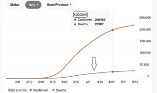
Fig 2. Cumulative distribution of the number of deaths for the time period between 21 February 2020 and 8 May 2020.

Statistical analysis
We now implement this model for the period from 21 February 2020 to 30 April 2020. The first category consists of 45 days (i.e. 45 × 1440 = 64,800 min), whereas the second one consists of 25 days (i.e. 25 × 1440 = 36,000 min). We thus have a two-component mixture model with 15,887 deaths for the category corresponding to 21 February 2020–5 April 2020 (see https://bing.com/covid/local/italy) and 12,080 deaths for the other category corresponding to 6 April 2020–30 April 2020 (calculated as total number of deaths up to 30 April 2020 = 27,967 – 15,887). The duration in minutes for each regime are D1 = 45 × 1440 = 64,800 (for 21 February 2020–5 April 2020) and D2 = 25 × 1440 = 36,000 (for 6 April 2020–30 April 2020).
The rates of deaths per minute λ1 and λ2 can be calculated as
Table 1. Observed Death Regimes and Calculated Parameters of the Mixture Model for the Period Between 21 February 2020 and 30 April 2020.
| Regime | Time period | Number of deaths | Duration of regime (minutes) | Rate per minute λ | Weighting factor w |
|---|---|---|---|---|---|
| 1 | 21 February 2020–5 April 2020 | 15,887 | 64,800 | 0.24517 | 0.357 |
| 2 | 6 April 2020–30 April 2020 | 12,080 | 36,000 | 0.33556 | 0.643 |
We also repeated the same reasoning for the time period between 21 February 2020 and 8 May 2020, with the same first category as before and a second category pertaining to data collected between 6 April 2020 and 8 May 2020. In that case, D1 = 64,800 min (as previously) and D2 = 47,520 min. Noticing that the number of deaths concerning the second regime is now 14,314 (30,201–15,887), we obtain
Table 2. Observed Death Regimes and Calculated Parameters of the Mixture Model for the Period Between 21 February 2020 and 8 May 2020.
| Regime | Time period | Number of deaths | Duration of regime (minutes) | Rate per minute λ | Weighting factor w |
|---|---|---|---|---|---|
| 1 | 21 February 2020–5 April 2020 | 15,887 | 64,800 | 0.24517 | 0.4231 |
| 2 | 6 April 2020–8 May 2020 | 14,314 | 47,520 | 0.30122 | 0.5769 |
Assessment of the model
The mixture model was assessed for the time period between 21 February 2020 and 8 May 2020 using a Kolmogorov–Smirnov goodness-of-fit test 5). Like in Mendoza-Rosas and De la Cruz Reyna 1, we also tested sensitivity in the quality of the fit by taking neighboring dates to 5 April 2020 (last day of the first regime selected by graphical inspection) as final dates for the first category and implementing again the Kolmogorov–Smirnov test.
Results
Using the aforementioned analysis, we now present in Tables 1, 2, and 3, the estimated parameters and probabilities of deaths within predetermined time intervals.
Table 3. Probabilities of Occurrence of at Least One Death in the Next t min.
| t | Cumulative Distribution 21 February 2020–30 April 2020 | Cumulative Distribution 21 February 2020–8 May 2020 |
|---|---|---|
| 2 | 0.467 | 0.4251 |
| 5 | 0.775 | 0.7479 |
| 10 | 0.94625 | 0.9352 |
| 15 | 0.9883 | 0.983 |
| 20 | 0.99657 | 0.9955 |
The cumulative distribution function is computed in the same way for values of t = 2, 5, 10, 15, and 20 min, for both periods, and results are presented in Table 3.
Discussion
Results presented in Table 3 are obtained using the hazard rates and the weighting factors, pertaining to the mixtures of exponentials that appear in Tables 1 and 2. These results show that the survival function, that is, the probability of exceeding some pre-specified t (= 1 – value from cumulative distribution) is slightly larger for the period between 21 February 2020 and 8 May 2020, which reflects the fact that the number of deaths occurring within the period between 1 May 2020 and 8 May 2020 have decreased in comparison to previous dates.
It is interesting to note that if we had used a single exponential distribution (instead of a mixture), we would then have obtained very close results to those provided by our mixture model for both periods, namely, 21 February 2020–30 April 2020 and 21 February 2020–8 May 2020. Indeed, let us consider the cdf F0*(t) of a single exponential distribution with parameter
Conclusions
In the present paper, we have proposed a method, based on mixtures of exponentials, for forecasting death hazards in populations hit by covid-19. In an earlier application to volcanic hazards, this method was shown to outperform standard techniques used in survival analysis. Two main advantages of the method are that it captures the different underlying categories (or regimes) suggested by the data and that it is quite handy and simple to implement, as component-wise hazard rates are readily obtained from the data. This is a very important asset in the context of covid-19 because, in contrast with volcanic hazards, repose periods are very short and so it would be useful to apply the method as many times as required in order to follow the course of the disease and thus help officials cope with difficulties concerning the health system at any stage of the pandemic. As an example, an application to the case of Italy was performed, and hazard rates were provided for two time periods for comparison reasons. The mixture model provided encouraging results, as it showed that a decrease in death numbers results, as expected, in larger values of the survival function.